Mean and Variance of Continuous Random Variables
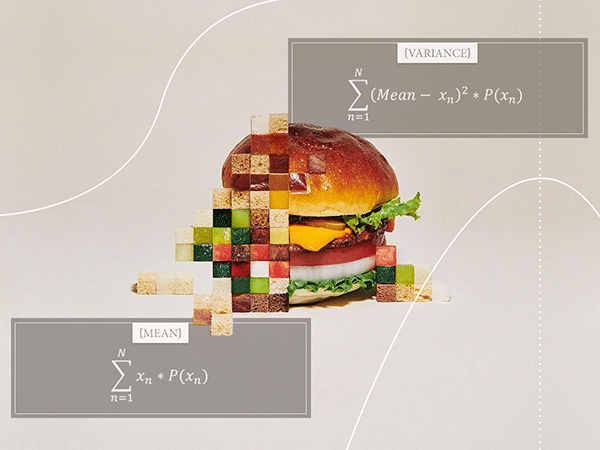
In my previous post I introduced you to probability distributions.
In short, a probability distribution is simply taking the whole probability mass of a random variable and distributing it across its possible outcomes. Since every random variable has a total probability mass equal to 1, this just means splitting the number 1 into parts and assigning each part to some element of the variable's sample space (informally speaking).
In this post I want to dig a little deeper into probability distributions and explore some of their properties. Namely, I want to talk about the measures of central tendency (the mean) and dispersion (the variance) of a probability distribution.
Relationship to previous posts
This post is a natural continuation of my previous 5 posts. In a way, it connects all the concepts I introduced in them:
- The Mean, The Mode, And The Median: Here I introduced the 3 most common measures of central tendency ("the three Ms") in statistics. I showed how to calculate each of them for a collection of values, as well as their intuitive interpretation. In the current post I'm going to focus only on the mean.
- The Law Of Large Numbers: Intuitive Introduction: This is a very important theorem in probability theory which links probabilities of outcomes to their relative frequencies of occurrence.
- An Intuitive Explanation Of Expected Value: In this post I showed how to calculate the long-term average of a random variable by multiplying each of its possible values by their respective probabilities and summing those products.
- The Variance: Measuring Dispersion: In this post I defined various measures of dispersion of a collection of values. In the current post I'm going to focus exclusively on variance.
- Introduction To Probability Distributions: Finally, in this post I talked about probability distributions which are assignments of probability masses or probability densities to each possible outcome of a random variable. Probability distributions are the main protagonist of the current post as well.
Without further ado, let's see how they all come together.
Introduction
Any finite collection of numbers has a mean and variance. In my previous posts I gave their respective formulas. Here's how you calculate the mean if we label each value in a collection as x1, x2, x3, x4, …, xn, …, xN:

If you're not familiar with this notation, take a look at my post dedicated to the sum operator. All this formula says is that to calculate the mean of N values, you first take their sum and then divide by N (their number).
And here's how you'd calculate the variance of the same collection:

So, you subtract each value from the mean of the collection and square the result. Then you add all these squared differences and divide the final sum by N. In other words, the variance is equal to the average squared difference between the values and their mean.
If you're dealing with finite collections, this is all you need to know about calculating their mean and variance. Finite collections include populations with finite size and samples of populations. But when working with infinite populations, things are slightly different.
Let me first define the distinction between samples and populations, as well as the notion of an infinite population.
Samples versus populations
A sample is simply a subset of outcomes from a wider set of possible outcomes, coming from a population.
For example, if you're measuring the heights of randomly selected students from some university, the sample is the subset of students you've chosen. The population could be all students from the same university. Or it could be all university students in the country. Or all university students in the world. The important thing is for all members of the sample to also be members of the wider population.
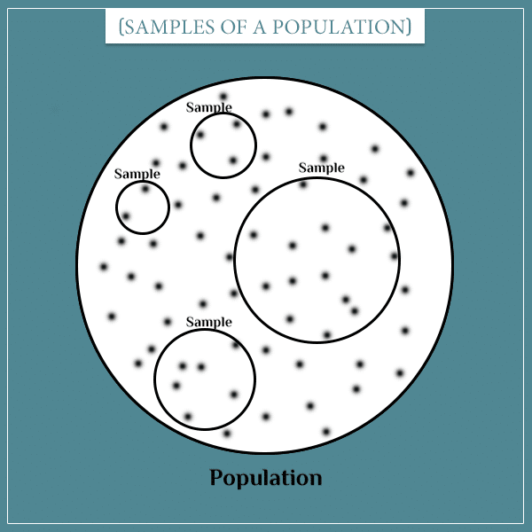
Samples obviously vary in size. Technically, even 1 element could be considered a sample. Whether a particular size is useful will, of course, depend on your purposes. Generally, the larger the sample is, the more representative you can expect it to be of the population it was drawn from.
The maximum size of a sample is clearly the size of the population. So, if your sample includes every member of the population, you are essentially dealing with the population itself.
It's also important to note that whether a collection of values is a sample or a population depends on the context. For example, if you're only interested in investigating something about students from University X, then the students of University X comprise the entirety of your population. On the other hand, if you want to learn something about all students of the country, then students from University X would be a sample of your target population.
Finite versus infinite populations
One difference between a sample and a population is that a sample is always finite in size. A population's size, on the other hand, could be finite but it could also be infinite. An infinite population is simply one with an infinite number of members.
Where do we come across infinite populations in real life? Well, we really don't. At any given moment, the number of any kind of entity is a fixed finite value. Even the number of atoms in the observable universe is a finite number. Infinite populations are more of a mathematical abstraction. They are born out of a hypothetical infinite repetition of a random process.
For example, if we assume that the universe will never die and our planet will manage to sustain life forever, we could consider the population of the organisms that ever existed and will ever exist to be infinite.
But where infinite populations really come into play is when we're talking about probability distributions. A probability distribution is something you could generate arbitrarily large samples from. In fact, in a way this is the essence of a probability distribution. You will remember from my introductory post that one way to view the probability distribution of a random variable is as the theoretical limit of its relative frequency distribution (as the number of repetitions approaches infinity).
Mean and variance of infinite populations
Like I said earlier, when dealing with finite populations, you can calculate the population mean or variance just like you do for a sample of that population. Namely, by taking into account all members of the population, not just a selected subset. For instance, to calculate the mean of the population, you would sum the values of every member and divide by the total number of members.
But what if we're dealing with a random variable which can continuously produce outcomes (like flipping a coin or rolling a die)? In this case we would have an infinite population and a sample would be any finite number of produced outcomes.
So, you can think of the population of outcomes of a random variable as an infinite sequence of outcomes produced according to its probability distribution. But how do we calculate the mean or the variance of an infinite sequence of outcomes?
The answer is actually surprisingly straightforward. Expected value to the rescue!

In my post on expected value, I defined it to be the sum of the products of each possible value of a random variable and that value's probability.
So, how do we use the concept of expected value to calculate the mean and variance of a probability distribution? Well, intuitively speaking, the mean and variance of a probability distribution are simply the mean and variance of a sample of the probability distribution as the sample size approaches infinity. In other words, the mean of the distribution is "the expected mean" and the variance of the distribution is "the expected variance" of a very large sample of outcomes from the distribution.
Let's see how this actually works.
The mean of a probability distribution
Let's say we need to calculate the mean of the collection {1, 1, 1, 3, 3, 5}.
According to the formula, it's equal to:
![]()
Using the distributive property of multiplication over addition, an equivalent way of expressing the left-hand side is:
- Mean = 1/6 + 1/6 + 1/6 + 3/6 + 3/6 + 5/6 = 2.33
Or:
- Mean = 3/6 * 1 + 2/6 * 3 + 1/6 * 5 = 2.33
That is, you take each unique value in the collection and multiply it by a factor of k / 6, where k is the number of occurrences of the value.
The mean and the expected value of a distribution are the same thing
Doesn't the ![]() factor kind of remind you of probabilities (by the classical definition of probability)? Notice, for example, that:
factor kind of remind you of probabilities (by the classical definition of probability)? Notice, for example, that:
![]()
Actually, the easiest way to interpret those as probabilities is if you imagine randomly drawing values from {1, 1, 1, 3, 3, 5} and replacing them immediately after. Then each of the three values will have a probability of ![]() of being drawn at every single trial.
of being drawn at every single trial.
With this process we're essentially creating a random variable out of the finite collection. And like all random variables, it has an infinite population of potential values, since you can keep drawing as many of them as you want. And naturally it has an underlying probability distribution.
If you repeat the drawing process M times, by the law of large numbers we know that the relative frequency of each of three values will be approaching k / 6 as M approaches infinity. So, using the ![]() representation of the mean formula, we can conclude the following:
representation of the mean formula, we can conclude the following:
- As M approaches infinity, the mean of a sample of size M will be approaching the mean of the original collection.
But now, take a closer look at the last expression. Do you notice that it is actually equivalent to the formula for expected value? Hence, we reach an important insight!
- The mean of a probability distribution is nothing more than its expected value.
If you remember, in my post on expected value I defined it precisely as the long-term average of a random variable. So, this should make a lot of sense.
Mean of discrete distributions
Well, here's the general formula for the mean of any discrete probability distribution with N possible outcomes:

As you can see, this is identical to the expression for expected value. Let's compare it to the formula for the mean of a finite collection:

Again, since N is a constant, using the distributive property, we can put the 1/N inside the sum operator. Then, each term will be of the form ![]() .
.

You could again interpret the ![]() factor as the probability of each value in the collection. I hope this gives you good intuition about the relationship between the two formulas.
factor as the probability of each value in the collection. I hope this gives you good intuition about the relationship between the two formulas.
Now let's use this to calculate the mean of an actual distribution. Let's go back to one of my favorite examples of rolling a die. The possible values are {1, 2, 3, 4, 5, 6} and each has a probability of ![]() . So, the mean (and expected value) of this distribution is:
. So, the mean (and expected value) of this distribution is:
![]()
Okay, the probability distribution's mean is 3.5, so what? Well, for one thing, if you generate a finite sample from the distribution, its mean will be approaching 3.5 as its size grows larger.
Let's see how this works with a simulation of rolling a die. The animation below shows 250 independent die rolls. The height of each bar represents the percentage of each outcome after each roll.
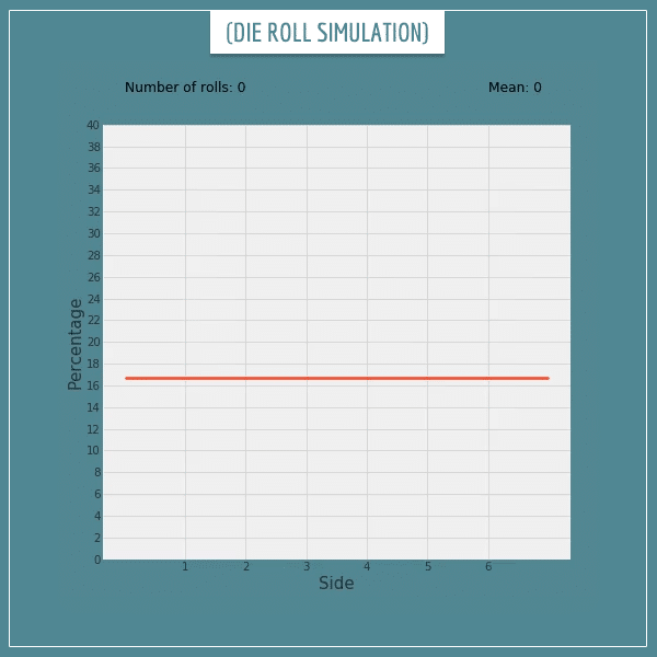
Click on the image to start/restart the animation.
Notice how the mean is fluctuating around the expected value 3.5 and eventually starts converging to it. If the sample grows to sizes above 1 million, the sample mean would be extremely close to 3.5.
Mean of continuous distributions
In my introductory post on probability distributions, I explained the difference between discrete and continuous random variables. Let's get a quick reminder about the latter.
In short, a continuous random variable's sample space is on the real number line. Since its possible outcomes are real numbers, there are no gaps between them (hence the term 'continuous'). The function underlying its probability distribution is called a probability density function.
In the post I also explained that exact outcomes always have a probability of 0 and only intervals can have non-zero probabilities. And, to calculate the probability of an interval, you take the integral of the probability density function over it.
Continuous random variables revisited
Let's look at the pine tree height example from the same post. The plot below shows its probability density function. The shaded area is the probability of a tree having a height between 14.5 and 15.5 meters.
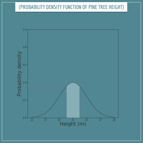
Let's use the notation f(x) for the probability density function (here x stands for height). Then the expression for the integral will be:
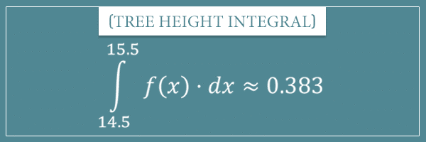
In the integrals section of my post related to 0 probabilities I said that one way to look at integrals is as the sum operator but for continuous random variables. That is, the expression above stands for the "infinite sum" of all values of f(x), where x is in the interval [14.5, 15.5]. Which happens to be approximately 0.383.
Because the total probability mass is always equal to 1, the following should also make sense:
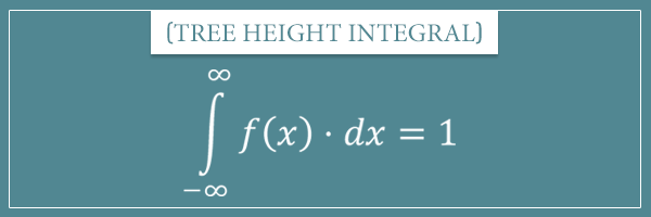
In fact, this formula holds in the general case for any continuous random variable. The integral of its probability density function from negative to positive infinity should always be equal to 1, in order to be consistent with Kolmogorov's axioms of probability.
You might be wondering why we're integrating from negative to positive infinity. What if the possible values of the random variable are only a subset of the real numbers? For example, a tree can't have a negative height, so negative real numbers are clearly not in the sample space. Another example would be a uniform distribution over a fixed interval like this:
![The probability density function over the interval [0, 1]](https://www.probabilisticworld.com/wp-content/uploads/2017/08/probability-density-function.png)
Well, this is actually not a problem, since we can simply assign 0 probability density to all values outside the sample space. This way they won't be contributing to the final value of the integral. That is, integrating from positive to negative infinity would give the same result as integrating only over the interval where the function is greater than zero.
The formula for the mean of a continuous random variable
So, after all this, it shouldn't be too surprising when I tell you that the mean formula for continuous random variables is the following:

Notice the similarities with the discrete version of the formula:

Instead of ![]() , here we have
, here we have ![]() . Essentially, we're multiplying every x by its probability density and "summing" the products.
. Essentially, we're multiplying every x by its probability density and "summing" the products.
And like in discrete random variables, here too the mean is equivalent to the expected value. And if we keep generating values from a probability density function, their mean will be converging to the theoretical mean of the distribution.
By the way, if you're not familiar with integrals, don't worry about the dx term. It means something like "an infinitesimal interval in x". Feel free to check out my post on zero probabilities for some intuition about it.
It's important to note that not all probability density functions have defined means. Although this topic is outside the scope of the current post, the reason is that the above integral doesn't converge to 1 for some probability density functions (it diverges to infinity). I am going to revisit this in future posts related to such distributions.
Well, this is it for means. If there's anything you're not sure you understand completely, feel free to ask in the comment section below.
Now let's take a look at the other main topic of this post: the variance.
The variance of a probability distribution
In this section I discuss the main variance formula of probability distributions. To see two useful (and insightful) alternative formulas, check out my latest post.
From the get-go, let me say that the intuition here is very similar to the one for means. The variance of a probability distribution is the theoretical limit of the variance of a sample of the distribution, as the sample's size approaches infinity.
The variance formula for a collection with N values is:

And here's the formula for the variance of a discrete probability distribution with N possible values:
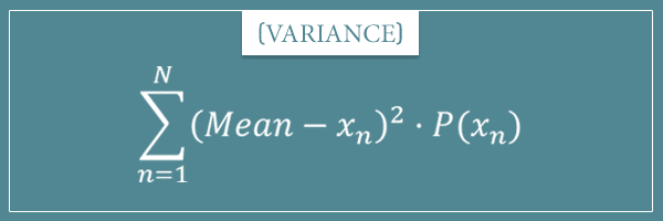
Do you see the analogy with the mean formula? Basically, the variance is the expected value of the squared difference between each value and the mean of the distribution. In the finite case, it is simply the average squared difference.
And, to complete the picture, here's the variance formula for continuous probability distributions:
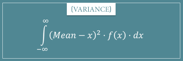
Again, notice the direct similarities with the discrete case. More specifically, the similarities between the terms:
![]()
![]()
In both cases, we're "summing" over all possible values of the random variable and multiplying each squared difference by the probability or probability density of the value. To get a better intuition, let's use the discrete formula to calculate the variance of a probability distribution. In fact, let's continue with the die rolling example.
The variance of a die roll
Let's do this step by step.
First, we need to subtract each value in {1, 2, 3, 4, 5, 6} from the mean of the distribution and take the square. Well, from the previous section, we already know that the mean is equal to 3.5. So, the 6 terms are:
![]()
![]()
![]()
![]()
![]()
![]()
Now we need to multiply each of the terms by the probability of the corresponding value and sum the products. Well, in this case they all have a probability of 1/6, so we can just use the distributive property:
![]()
Which is equal to:
![]()
So, the variance of this probability distribution is approximately 2.92.
To get an intuition about this, let's do another simulation of die rolls. I wrote a short code that generates 250 random rolls and calculates the running relative frequency of each outcome and the variance of the sample after each roll. Click on the image below to see this simulation animated:
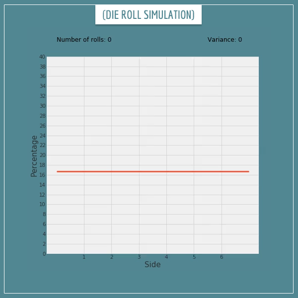
Click on the image to start/restart the animation.
You see how the running variance keeps fluctuating around the theoretical expectation of 2.92? It doesn't quite converge after only 250 rolls, but if we keep increasing the number of rolls, eventually it will.
The bottom line is that, as the relative frequency distribution of a sample approaches the theoretical probability distribution it was drawn from, the variance of the sample will approach the theoretical variance of the distribution.
Mean and variance of functions of random variables
This section was added to the post on the 7th of November, 2020.
To conclude this post, I want to show you something very simple and intuitive that will be useful for you in many contexts.
By now you know the general formulas for calculating the mean and variance of a probability distribution, both for discrete and continuous cases. These formulas work with the elements of the sample space associated with the distribution. To calculate the mean, you're multiplying every element by its probability (and summing or integrating these products). Similarly, for the variance you're multiplying the squared difference between every element and the mean by the element's probability.
Now, imagine taking the sample space of a random variable X and passing it to some function. Let's call this function g(x). Notice that by doing so you obtain a new random variable Y which has different elements in its sample space. For example, if ![]() and X = {1, 2, 3}, then Y = {1, 4, 9}.
and X = {1, 2, 3}, then Y = {1, 4, 9}.
However, even though the values are different, their probabilities will be identical to the probabilities of their corresponding elements in X:
![]()
Which means that you can calculate the mean and variance of Y by plugging in the probabilities of X into the formulas. For example, if we stick with the ![]() example and define
example and define ![]() , the formulas for the mean and variance of Y would be:
, the formulas for the mean and variance of Y would be:
![Rendered by QuickLaTeX.com \[\textrm{Mean}(Y) = \sum_{n=1}^{N} y_n \cdot P(y_n) = \sum_{n=1}^{N} x_n^3 \cdot P(x_n)\]](https://www.probabilisticworld.com/wp-content/ql-cache/quicklatex.com-b8690289dcf319041ceb435c15c2c7fb_l3.png)
![Rendered by QuickLaTeX.com \[\textrm{Variance}(Y) = \sum_{n=1}^{N} (\textrm{Mean}(Y) - y_n)^2 \cdot P(y_n) = \sum_{n=1}^{N} (\textrm{Mean}(X^3) - x_n^3)^2 \cdot P(x_n)\]](https://www.probabilisticworld.com/wp-content/ql-cache/quicklatex.com-7daf8e9bc46f2f29d1b79052d994b379_l3.png)
In the general case, for any discrete random variable X and any function g(x):
![Rendered by QuickLaTeX.com \[\textrm{Mean}(g(X)) = \sum_{n=1}^{N} g(x_n) \cdot P(x_n)\]](https://www.probabilisticworld.com/wp-content/ql-cache/quicklatex.com-f0f21700da0be410d760e8e74923260c_l3.png)
![Rendered by QuickLaTeX.com \[\textrm{Variance}(g(X)) = \sum_{n=1}^{N} (\textrm{Mean}(g(X)) - g(x_n))^2 \cdot P(x_n)\]](https://www.probabilisticworld.com/wp-content/ql-cache/quicklatex.com-6567175fadd67b35db571b806c58590d_l3.png)
And the continuous case is analogous. If we have a continuous random variable X with a probability density function f(x), then for any function g(x):
![]()
![]()
Another die roll example
One application of what I just showed you would be in calculating the mean and variance of your expected monetary wins/losses if you're betting on outcomes of a random variable. The association between outcomes and their monetary value would be represented by a function.
For example, say someone offers you the following game. You will roll a regular six-sided die with sides labeled 1, 2, 3, 4, 5, and 6. If the side that comes up is an odd number, you win an amount (in dollars) equal to the cube of the number. And if it's an even number, you lose the square of the number. We can represent these payouts with the following function:
![Rendered by QuickLaTeX.com \[ g(x) = \begin{cases}x^3 & x \in \{1, 3, 5\} \\-x^2 & x \in \{2, 4, 6\}\end{cases}\]](https://www.probabilisticworld.com/wp-content/ql-cache/quicklatex.com-c915df3e546eca074708fd4fae1cba63_l3.png)
Using the mean formula:
![Rendered by QuickLaTeX.com \[\textrm{Mean}(g(X)) = \sum_{n=1}^{N} g(x_n) \cdot P(x_n)\]](https://www.probabilisticworld.com/wp-content/ql-cache/quicklatex.com-f0f21700da0be410d760e8e74923260c_l3.png)
![]()
To apply the variance formula, let's first calculate the squared differences using the mean we just calculated:
![]()
![]()
![]()
![]()
![]()
![]()
Now let's apply the formula:
![Rendered by QuickLaTeX.com \[\textrm{Variance}(g(X)) = \sum_{n=1}^{N} (\textrm{Mean}(g(X)) - g(x_n))^2 \cdot P(x_n)\]](https://www.probabilisticworld.com/wp-content/ql-cache/quicklatex.com-6567175fadd67b35db571b806c58590d_l3.png)
![]()
Notice that I didn't put in any units because technically the variance would need to be in "squared dollars", which would be a little confusing.
Summary
One of my goals in this post was to show the fundamental relationship between the following concepts from probability theory:
- Mean and variance
- The law of large numbers
- Expected value
- Probability distributions
I also introduced the distinction between samples and populations. And more importantly, the difference between finite and infinite populations. I tried to give the intuition that, in a way, a probability distribution represents an infinite population of values drawn from it. And that the mean and variance of a probability distribution are essentially the mean and variance of that infinite population.
In other words, they are the theoretical expected mean and variance of a sample of the probability distribution, as the size of the sample approaches infinity.
The main takeaway from this post are the mean and variance formulas for finite collections of values compared to their variants for discrete and continuous probability distributions. I hope I managed to give you a good intuitive feel for the connection between them. Let's take a final look at these formulas.
These are the formulas for the mean:


And here are the formulas for the variance:


Maybe take some time to compare these formulas to make sure you see the connection between them.
Finally, in the last section I talked about calculating the mean and variance of functions of random variables. For an arbitrary function g(x), the mean and variance of a function of a discrete random variable X are given by the following formulas:
![Rendered by QuickLaTeX.com \[\textrm{Mean}(g(X)) = \sum_{n=1}^{N} g(x_n) \cdot P(x_n)\]](https://www.probabilisticworld.com/wp-content/ql-cache/quicklatex.com-f0f21700da0be410d760e8e74923260c_l3.png)
![Rendered by QuickLaTeX.com \[\textrm{Variance}(g(X)) = \sum_{n=1}^{N} (\textrm{Mean}(g(X)) - g(x_n))^2 \cdot P(x_n)\]](https://www.probabilisticworld.com/wp-content/ql-cache/quicklatex.com-6567175fadd67b35db571b806c58590d_l3.png)
And for a continuous random variable X:
![]()
![]()
Anyway, I hope you found this post useful. If you had any difficulties with any of the concepts or explanations, please leave your questions in the comment section.
phillipsanned2001.blogspot.com
Source: https://www.probabilisticworld.com/mean-variance-probability-distributions/
0 Response to "Mean and Variance of Continuous Random Variables"
Post a Comment